TensorRT-Int8量化详解

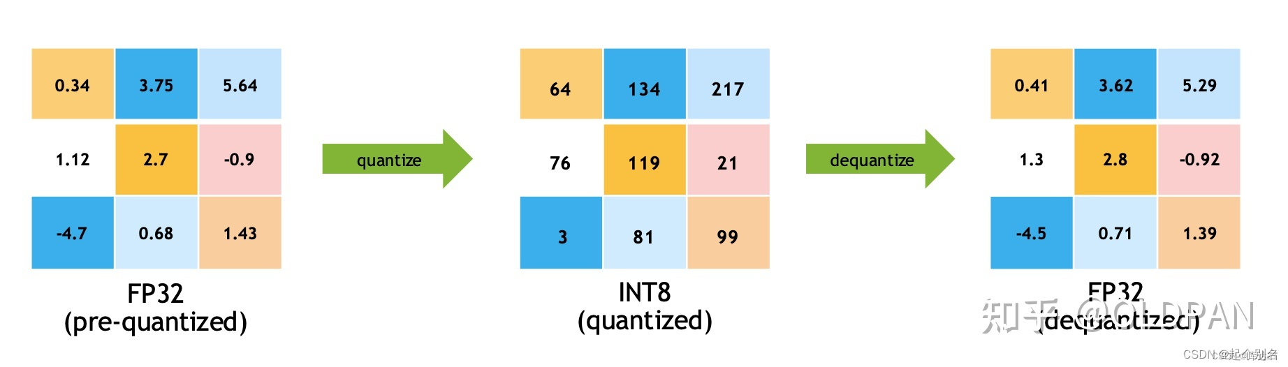
int8量化是利用int8乘法替换float32乘法实现性能加速的一种方法

对于常规模型有：y = kx + b，此时x、k、b都是float32, 对于kx的计算使用float32的乘法
对于int8模型有：y = tofp32(toint8(k) * toint8(x)) + b，其中int8 * int8结果为int16
因此int8模型解决的问题是如何将float32合理的转换为int8，使得精度损失最小
也因此，经过int8量化的精度会受到影响

Int8量化步骤：
1. 配置setFlag nvinfer1::BuilderFlag::kINT8
2. 实现Int8EntropyCalibrator类并继承自IInt8EntropyCalibrator2
3. 实例化Int8EntropyCalibrator并且设置到config.setInt8Calibrator
4. Int8EntropyCalibrator的作用，是读取并预处理图像数据作为输入
- 标定过程的理解：对于输入图像A，使用FP32推理后得到P1再用INT8推理得到P2，调整int8权重使得P1与P2足够的接近
- 因此标定时需要使用一些图像，正常发布时，使用100张图左右即可

创建模型，py推理:

gen-onnx.py

import torch
import torchvision
import cv2
import numpy as np
 
 
class Classifier(torch.nn.Module):
    def __init__(self):
        super().__init__()
        self.backbone = torchvision.models.resnet18(pretrained=True)
        
    def forward(self, x):
        feature     = self.backbone(x)
        probability = torch.softmax(feature, dim=1)
        return probability
        
 
imagenet_mean = [0.485, 0.456, 0.406]
imagenet_std  = [0.229, 0.224, 0.225]
 
image = cv2.imread("workspace/kej.jpg")
image = cv2.resize(image, (224, 224))            # resize
image = image[..., ::-1]                         # BGR -> RGB
image = image / 255.0
image = (image - imagenet_mean) / imagenet_std   # normalize
image = image.astype(np.float32)                 # float64 -> float32
image = image.transpose(2, 0, 1)                 # HWC -> CHW
image = np.ascontiguousarray(image)              # contiguous array memory
image = image[None, ...]                         # CHW -> 1CHW
image = torch.from_numpy(image)                  # numpy -> torch
model = Classifier().eval()
 
with torch.no_grad():
    probability   = model(image)
    
predict_class = probability.argmax(dim=1).item()
confidence    = probability[0, predict_class]
 
labels = open("workspace/labels.imagenet.txt").readlines()
labels = [item.strip() for item in labels]
 
print(f"Predict: {predict_class}, {confidence}, {labels[predict_class]}")
 
dummy = torch.zeros(1, 3, 224, 224)
torch.onnx.export(
    model, (dummy,), "workspace/classifier.onnx", 
    input_names=["image"], 
    output_names=["prob"], 
    dynamic_axes={"image": {0: "batch"}, "prob": {0: "batch"}},
    opset_version=11
)

这里采用的是一个分类器模型：

class Classifier(torch.nn.Module):
    def __init__(self):
        super().__init__()
        self.backbone = torchvision.models.resnet18(pretrained=True)
        
    def forward(self, x):
        feature     = self.backbone(x)
        probability = torch.softmax(feature, dim=1)
        return probability

使用resnet18作为backbone，pretrained=True将预训练模型作为初始化。返回softmax结果。

后面的就是图像的预处理过程，这部分可以让我们想到之前的warpaffine过程。

紧接着做一个推理过程，不计算梯度可以提高运行效率：

 
with torch.no_grad():
    probability   = model(image)

使用resnet18作为backbone，pretrained=True将预训练模型作为初始化。返回softmax结果。

后面的就是图像的预处理过程，这部分可以让我们想到之前的warpaffine过程。

紧接着做一个推理过程，不计算梯度可以提高运行效率：

 
with torch.no_grad():
    probability   = model(image)

   
predict_class = probability.argmax(dim=1).item()
confidence    = probability[0, predict_class]
 
labels = open("workspace/labels.imagenet.txt").readlines()
labels = [item.strip() for item in labels]
 
print(f"Predict: {predict_class}, {confidence}, {labels[predict_class]}")

将结果取出，读取名为"labels.imagenet.txt"的文件，并将每一行的内容存储在一个列表中。strip()函数用于删除每个元素前后的空白字符。所以，最终得到的列表包含了该文件中的所有标签。最后输出结果。

dummy = torch.zeros(1, 3, 224, 224)
torch.onnx.export(
    model, (dummy,), "workspace/classifier.onnx", 
    input_names=["image"], 
    output_names=["prob"], 
    dynamic_axes={"image": {0: "batch"}, "prob": {0: "batch"}},
    opset_version=11
)

最后将这个模型导出为一个onnx，

dynamic_axes用于指定图中哪些维度应该被视为动态维度，这里只有batch为动态。

opset_version参数指定了所使用的ONNX的版本号，这里使用的是版本11。

TRT标定量化推理：

main.cpp:

build_model：

bool build_model(){
 
    if(exists("engine.trtmodel")){
        printf("Engine.trtmodel has exists.\n");
        return true;
    }
 
TRTLogger logger;
 
    // 这是基本需要的组件
    auto builder = make_nvshared(nvinfer1::createInferBuilder(logger));
    auto config = make_nvshared(builder->createBuilderConfig());
 
    // createNetworkV2(1)表示采用显性batch size，新版tensorRT(>=7.0)时，不建议采用0非显性batch size
    // 因此贯穿以后，请都采用createNetworkV2(1)而非createNetworkV2(0)或者createNetwork
    auto network = make_nvshared(builder->createNetworkV2(1));
 
    // 通过onnxparser解析器解析的结果会填充到network中，类似addConv的方式添加进去
    auto parser = make_nvshared(nvonnxparser::createParser(*network, logger));
    if(!parser->parseFromFile("classifier.onnx", 1)){
        printf("Failed to parse classifier.onnx\n");
 
        // 注意这里的几个指针还没有释放，是有内存泄漏的，后面考虑更优雅的解决
        return false;
    }
    
    int maxBatchSize = 10;
    printf("Workspace Size = %.2f MB\n", (1 << 28) / 1024.0f / 1024.0f);
    config->setMaxWorkspaceSize(1 << 28);
 
    // 如果模型有多个执行上下文，则必须多个profile
    // 多个输入共用一个profile
    auto profile = builder->createOptimizationProfile();
    auto input_tensor = network->getInput(0);
    auto input_dims = input_tensor->getDimensions();
 
    input_dims.d[0] = 1;

到这里的步骤和之前的都没区别，make_nvshared是将他设定为了一个智能指针一样的东西，就可以自动destroy。

开始量化：

之后 config->setFlag(nvinfer1::BuilderFlag::kINT8);，这是咱们开头说过的int8量化的第一步

 config->setFlag(nvinfer1::BuilderFlag::kINT8);
 
    auto preprocess = [](
        int current, int count, const std::vector<std::string>& files, 
        nvinfer1::Dims dims, float* ptensor
    ){
        printf("Preprocess %d / %d\n", count, current);
 
        // 标定所采用的数据预处理必须与推理时一样
        int width = dims.d[3];
        int height = dims.d[2];
        float mean[] = {0.406, 0.456, 0.485};
        float std[]  = {0.225, 0.224, 0.229};
 
        for(int i = 0; i < files.size(); ++i){
 
            auto image = cv::imread(files[i]);
            cv::resize(image, image, cv::Size(width, height));
            int image_area = width * height;
            unsigned char* pimage = image.data;
            float* phost_b = ptensor + image_area * 0;
            float* phost_g = ptensor + image_area * 1;
            float* phost_r = ptensor + image_area * 2;
            for(int i = 0; i < image_area; ++i, pimage += 3){
                // 注意这里的顺序rgb调换了
                *phost_r++ = (pimage[0] / 255.0f - mean[0]) / std[0];
                *phost_g++ = (pimage[1] / 255.0f - mean[1]) / std[1];
                *phost_b++ = (pimage[2] / 255.0f - mean[2]) / std[2];
            }
            ptensor += image_area * 3;
        }
    };

之后的一段就是和python里的差不多的顺序了，先保存标准差和均值，之后用cv读进来resize为（224，224）这都是在onnx里设定好了的dim。之后做一个rgb和bgr的调换。

BGRBGRBGR ------->>> BBBGGGRRR

（在一些特定的硬件平台或者处理器架构上，例如Intel x86架构，使用BGR格式可以更高效地进行图像处理操作。这是因为x86体系结构中关于字节序（Endianness）的规定，在内存中低序（little-endian）存储方式下，处理器对字节的访问方式有一定的影响。同时，许多图像处理库和算法也使用BGR格式进行计算和处理。）

之后实例化Int8EntropyCalibrator类，这也是我们第二个步骤所提到的。

 // 配置int8标定数据读取工具
    shared_ptr<Int8EntropyCalibrator> calib(new Int8EntropyCalibrator(
        {"kej.jpg"}, input_dims, preprocess
    ));
    config->setInt8Calibrator(calib.get());

Int8EntropyCalibrator类主要关注：

1、getBatchSize，告诉引擎，这次标定的batch是多少

    int getBatchSize() const noexcept {
        return dims_.d[0];
    }

这里的dims.d[0]其实就是我们刚刚build_model里设置的
input_dims.d[0] = 1;

2、getBatch，告诉引擎，这次标定的输入数据是什么，把指针赋值给bindings即可，返回false表示没有数据了

 
    bool next() {
        int batch_size = dims_.d[0];
        if (cursor_ + batch_size > allimgs_.size())
            return false;
 
        for(int i = 0; i < batch_size; ++i)
            files_[i] = allimgs_[cursor_++];
 
        if(tensor_host_ == nullptr){
            size_t volumn = 1;
            for(int i = 0; i < dims_.nbDims; ++i)
                volumn *= dims_.d[i];
            
            bytes_ = volumn * sizeof(float);
            checkRuntime(cudaMallocHost(&tensor_host_, bytes_));
            checkRuntime(cudaMalloc(&tensor_device_, bytes_));
        }
 
        preprocess_(cursor_, allimgs_.size(), files_, dims_, tensor_host_);
        checkRuntime(cudaMemcpy(tensor_device_, tensor_host_, bytes_, cudaMemcpyHostToDevice));
        return true;
    }
 
    bool getBatch(void* bindings[], const char* names[], int nbBindings) noexcept {
        if (!next()) return false;
        bindings[0] = tensor_device_;
        return true;
    }

这里的file就是我们放入的图片， files_[i] = allimgs_[cursor_++];读进来，而且这里只有一张图是因为在 shared_ptr<Int8EntropyCalibrator> calib(new Int8EntropyCalibrator(
{"kej.jpg"}, input_dims, preprocess ));只放了一张keji图片进来。

3、readCalibrationCache，若从缓存文件加载标定信息，则可避免读取文件和预处理，若该函数返回空指针则表示没有缓存，程序会重新通过getBatch重新计算

    const void* readCalibrationCache(size_t& length) noexcept {
        if (fromCalibratorData_) {
            length = this->entropyCalibratorData_.size();
            return this->entropyCalibratorData_.data();
        }
 
        length = 0;
        return nullptr;
    }

这个常常用在多次标定的情况下，可以避免多次重新计算

4、writeCalibrationCache，当标定结束后，会调用该函数，我们可以储存标定后的缓存结果，多次标定可以使用该缓存实现加速

    virtual void writeCalibrationCache(const void* cache, size_t length) noexcept {
        entropyCalibratorData_.assign((uint8_t*)cache, (uint8_t*)cache + length);
    }

这个就是自动帮你缓存

之后用

    config->setInt8Calibrator(calib.get());

对其进行实例化。

存储：

   // 配置最小允许batch
    input_dims.d[0] = 1;
    profile->setDimensions(input_tensor->getName(), nvinfer1::OptProfileSelector::kMIN, input_dims);
    profile->setDimensions(input_tensor->getName(), nvinfer1::OptProfileSelector::kOPT, input_dims);
 
    // 配置最大允许batch
    // if networkDims.d[i] != -1, then minDims.d[i] == optDims.d[i] == maxDims.d[i] == networkDims.d[i]
    input_dims.d[0] = maxBatchSize;
    profile->setDimensions(input_tensor->getName(), nvinfer1::OptProfileSelector::kMAX, input_dims);
    config->addOptimizationProfile(profile);
 
    auto engine = make_nvshared(builder->buildEngineWithConfig(*network, *config));
    if(engine == nullptr){
        printf("Build engine failed.\n");
        return false;
    }
 
    // 将模型序列化，并储存为文件
    auto model_data = make_nvshared(engine->serialize());
    FILE* f = fopen("engine.trtmodel", "wb");
    fwrite(model_data->data(), 1, model_data->size(), f);
    fclose(f);
 
    f = fopen("calib.txt", "wb");
    auto calib_data = calib->getEntropyCalibratorData();
    fwrite(calib_data.data(), 1, calib_data.size(), f);
    fclose(f);
 
    // 卸载顺序按照构建顺序倒序
    printf("Done.\n");
    return true;
}

这里会多一步：

      f = fopen("calib.txt", "wb");
        auto calib_data = calib->getEntropyCalibratorData();
        fwrite(calib_data.data(), 1, calib_data.size(), f);
        fclose(f);

将缓存储存下来

推理过程：

整体代码如下：

 
void inference(){
 
    TRTLogger logger;
    auto engine_data = load_file("engine.trtmodel");
    auto runtime   = make_nvshared(nvinfer1::createInferRuntime(logger));
    auto engine = make_nvshared(runtime->deserializeCudaEngine(engine_data.data(), engine_data.size()));
    if(engine == nullptr){
        printf("Deserialize cuda engine failed.\n");
        runtime->destroy();
        return;
    }
 
    cudaStream_t stream = nullptr;
    checkRuntime(cudaStreamCreate(&stream));
    auto execution_context = make_nvshared(engine->createExecutionContext());
 
    int input_batch   = 1;
    int input_channel = 3;
    int input_height  = 224;
    int input_width   = 224;
    int input_numel   = input_batch * input_channel * input_height * input_width;
    float* input_data_host   = nullptr;
    float* input_data_device = nullptr;
    checkRuntime(cudaMallocHost(&input_data_host, input_numel * sizeof(float)));
    checkRuntime(cudaMalloc(&input_data_device, input_numel * sizeof(float)));
 
    ///
    // image to float
    auto image = cv::imread("kej.jpg");
    float mean[] = {0.406, 0.456, 0.485};
    float std[]  = {0.225, 0.224, 0.229};
 
        //图像存储BGRBGRBGR ---->  BBBGGGRRR
    // 对应于pytorch的代码部分
    cv::resize(image, image, cv::Size(input_width, input_height));
    int image_area = image.cols * image.rows; //图像面积
    unsigned char* pimage = image.data; //图像像素数据
    float* phost_b = input_data_host + image_area * 0; //获取B的起始位置
    float* phost_g = input_data_host + image_area * 1; // 获取G的起始位置
    float* phost_r = input_data_host + image_area * 2; //获取R的起始位置
    for(int i = 0; i < image_area; ++i, pimage += 3){
        // 注意这里的顺序rgb调换了
        *phost_r++ = (pimage[0] / 255.0f - mean[0]) / std[0];
        *phost_g++ = (pimage[1] / 255.0f - mean[1]) / std[1];
        *phost_b++ = (pimage[2] / 255.0f - mean[2]) / std[2];
    }
    ///
    checkRuntime(cudaMemcpyAsync(input_data_device, input_data_host, input_numel * sizeof(float), cudaMemcpyHostToDevice, stream));;
 
    // 3x3输入，对应3x3输出
    const int num_classes = 1000;
    float output_data_host[num_classes];
    float* output_data_device = nullptr;
    checkRuntime(cudaMalloc(&output_data_device, sizeof(output_data_host)));
 
    // 明确当前推理时，使用的数据输入大小
    auto input_dims = execution_context->getBindingDimensions(0);
    input_dims.d[0] = input_batch;
 
    execution_context->setBindingDimensions(0, input_dims);
    float* bindings[] = {input_data_device, output_data_device};
    bool success      = execution_context->enqueueV2((void**)bindings, stream, nullptr);
    checkRuntime(cudaMemcpyAsync(output_data_host, output_data_device, sizeof(output_data_host), cudaMemcpyDeviceToHost, stream));
    checkRuntime(cudaStreamSynchronize(stream));
 
    float* prob = output_data_host;
    int predict_label = std::max_element(prob, prob + num_classes) - prob;
    auto labels = load_labels("labels.imagenet.txt");
    auto predict_name = labels[predict_label];
    float confidence  = prob[predict_label];
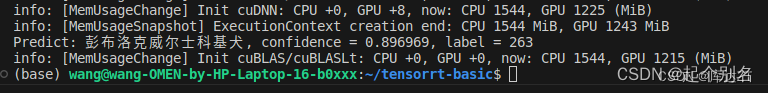
    printf("Predict: %s, confidence = %f, label = %d\n", predict_name.c_str(), confidence, predict_label);
 
    checkRuntime(cudaStreamDestroy(stream));
    checkRuntime(cudaFreeHost(input_data_host));
    checkRuntime(cudaFree(input_data_device));
    checkRuntime(cudaFree(output_data_device));
}

首先对于前面的内容和fp32一模一样：

    TRTLogger logger;
    auto engine_data = load_file("engine.trtmodel");
    auto runtime   = make_nvshared(nvinfer1::createInferRuntime(logger));
    auto engine = make_nvshared(runtime->deserializeCudaEngine(engine_data.data(), engine_data.size()));
    if(engine == nullptr){
        printf("Deserialize cuda engine failed.\n");
        runtime->destroy();
        return;
    }
 
    cudaStream_t stream = nullptr;
    checkRuntime(cudaStreamCreate(&stream));
    auto execution_context = make_nvshared(engine->createExecutionContext());
 
    int input_batch   = 1;
    int input_channel = 3;
    int input_height  = 224;
    int input_width   = 224;
    int input_numel   = input_batch * input_channel * input_height * input_width;
    float* input_data_host   = nullptr;
    float* input_data_device = nullptr;
    checkRuntime(cudaMallocHost(&input_data_host, input_numel * sizeof(float)));
    checkRuntime(cudaMalloc(&input_data_device, input_numel * sizeof(float)));

加载模型反序列化，创建流，创建一个上下文，再指定batch和channel，weight ， height

在推理阶段也要和标定时作一样的处理

   // image to float
    auto image = cv::imread("kej.jpg");
    float mean[] = {0.406, 0.456, 0.485};
    float std[]  = {0.225, 0.224, 0.229};
 
    // 对应于pytorch的代码部分
    cv::resize(image, image, cv::Size(input_width, input_height));
    int image_area = image.cols * image.rows;
    unsigned char* pimage = image.data;
    float* phost_b = input_data_host + image_area * 0;
    float* phost_g = input_data_host + image_area * 1;
    float* phost_r = input_data_host + image_area * 2;
    for(int i = 0; i < image_area; ++i, pimage += 3){
        // 注意这里的顺序rgb调换了
        *phost_r++ = (pimage[0] / 255.0f - mean[0]) / std[0];
        *phost_g++ = (pimage[1] / 255.0f - mean[1]) / std[1];
        *phost_b++ = (pimage[2] / 255.0f - mean[2]) / std[2];
    }
    ///
    checkRuntime(cudaMemcpyAsync(input_data_device, input_data_host, input_numel * sizeof(float), cudaMemcpyHostToDevice, stream));

之后用max_element找到最大值的索引并输出，推理结束：

 
    // 3x3输入，对应3x3输出
    const int num_classes = 1000;
    float output_data_host[num_classes];
    float* output_data_device = nullptr;
    checkRuntime(cudaMalloc(&output_data_device, sizeof(output_data_host)));
 
    // 明确当前推理时，使用的数据输入大小
    auto input_dims = execution_context->getBindingDimensions(0);
    input_dims.d[0] = input_batch;
 
    execution_context->setBindingDimensions(0, input_dims);
    float* bindings[] = {input_data_device, output_data_device};
    bool success      = execution_context->enqueueV2((void**)bindings, stream, nullptr);
    checkRuntime(cudaMemcpyAsync(output_data_host, output_data_device, sizeof(output_data_host), cudaMemcpyDeviceToHost, stream));
    checkRuntime(cudaStreamSynchronize(stream));
 
    float* prob = output_data_host;
    int predict_label = std::max_element(prob, prob + num_classes) - prob;
    auto labels = load_labels("labels.imagenet.txt");
    auto predict_name = labels[predict_label];
    float confidence  = prob[predict_label];
    printf("Predict: %s, confidence = %f, label = %d\n", predict_name.c_str(), confidence, predict_label);
 
    checkRuntime(cudaStreamDestroy(stream));
    checkRuntime(cudaFreeHost(input_data_host));
    checkRuntime(cudaFree(input_data_device));
    checkRuntime(cudaFree(output_data_device));
}

总结：

Int8量化类似于一个黑盒子，有一点蒸馏的感觉，用int8逼近fp32的推理结果。

我们只需要按照步骤设定好参数之后set就可以，并不需要特别关注于他是怎么修改权重的

番外：量化操作理论篇：

如何正确导出ONNX

对于任何用到shape、size返回值的参数时，例如：tensor.view(tensor..size(0),-1)这类操作，避免直接使用tensor.size的返回值，而是加上int转换，tensor.view(int(tensor.size(0)),-1)
对于nn.Upsample或nn.functional.interpolate函数，使用scale_factor指定倍率，而不是使用size参数指定大小
对于reshape、view操作时，-1的指定请放到batch维度。其他维度可以计算出来即可。batch维度禁止指定为大于-1的明确数字
torch.onnx.export指定dynamic_axes参数，并且只指定batch维度，不指定其他维度。我们只需要动态batch,相对动态的宽高有其他方案
使用Opset_Version=11,不要低于11，（低于的话为unsample，不是resize）
避免使用inplace操作

这些做法的必要性体现在，简化过程的复杂度，去掉gather、shape类的节点。

例如：将reshape的batch的维度指定为-1

# bs, _, ny, nx = x[i].shape  # x(bs,255,20,20) to x(bs,3,20,20,85)
  bs, _, ny, nx = map(int,x[i].shape)
# x[i] = x[i].view(bs, self.na, self.no, ny, nx).permute(0, 1, 3, 4, 2).contiguous()
  x[i] = x[i].view(-1, self.na, self.no, ny, nx).permute(0, 1, 3, 4, 2).contiguous()
 
 
# z.append(y.view(-1, int(y.size(1)*y.size(2)*y.size(3)), self.no))
  z.append(y.view(-1, int(torch.prod(torch.tensor(y.shape[1:-1]))), self.no))

去除多余的输出：

return x if self.training else torch.cat(z, 1)

高性能注意点

单模型推理时的性能问题：

尽量使得GPU高密集度运行，避免出现CPU、GPU相互交换运行
尽可能使tensorRT:运行多个batch数据。与第一点相合
预处理尽量cuda化，例如图像需要做normalize、reisze、warpaffine、bgr2rgb等，在这里，采用cuda核实现warpaffine+normalize等操作，集中在一起性能
后处理尽量cuda化，例如decode、nms等。在这里用cuda核实现了decode和nms
善于使用cudaStream,将操作加入流中，采用异步操作避免等待
内存复用

系统级别的性能问题：